Post-Training Quantization of Language Models

During my end-of-study internship, I worked as an operational consultant, sent on a technical mission to the scientific research department of a large company. This post is summary of my end-of-study report, about the work I did on the quantization of Large Language Models (LLM) for this company.

Context

The client needed a pipeline for summarizing research articles as part of their technology watch. The solution proposed and chosen was to use Large Language Models (LLM), without recourse to external solutions, in order to preserve confidentiality and control costs. Initially, I set up a cloud-based working environment on AWS to facilitate the deployment and management of the resources required for the project. I then benchmarked the available open-source solutions to assess their relevance to our specific needs. The choice of tools was a crucial element of my work, and I opted for cost-efficient hardware solutions that met our performance requirements. All the models selected were approved by the relevant legal regulations. Optimization was an iterative process, where I sought to achieve the best possible results by fine-tuning the pipeline parameters. Finally, to improve prompt size and processing speed on reasonable GPUs, I used the Post-Training Quantization technique.

The evolution of language models

Historical Background

The evolution of language models has been marked by several crucial milestones, reflecting advances in the fields of computer science and machine learning. Early approaches, such as n-gram models, focused on predicting words based on their immediate contexts (Ganesan et al., 2012). However, these approaches were limited in terms of understanding the wider context and complex relationships between words. The introduction of artificial neural networks paved the way for more sophisticated models (Bengio et al., 2003) capable of capturing longer-range dependencies in text. Recurrent Neural Networks (RNNs) were among the first to be used to model sequences, taking word order into account. However, RNNs suffered from the vanishing gradient problem (Pascanu et al., 2012), limiting their training capabilities. Subsequent advances, such as the Long Short-Term Memory models (LSTM) (Hochreiter and Schmidhuber, 1997; Jozefowicz et al., 2016) have shifted these limitations on memory. Indeed, these recurrent models process input and output sequence symbols step by step. Each step creates a series of hidden states \(h_t\) based on the previous hidden state \(h_{t-1}\). This sequential approach makes parallelization impossible, which complicates training when the sequence becomes very long.

Transformers

Transformers, successfully introduced by the publication “Attention Is All You Need” (Vaswani et al., 2017), revolutionized language models by using attention mechanisms to capture word relationships more efficiently and avoiding the recurrence of previous solutions. This evolution culminated in pre-trained language models such as BERT (Devlin et al., 2019) (Google) and GPT (Radford and Narasimhan, 2018) (OpenAI), which dramatically improved the ability to comprehend and generate text. The academic and scientific world took the measure of the impact of this new technology in December 2022, when OpenAI released ChatGPT, a conversational agent powered by their GPT-3.5 model, whose precise architecture and number of parameters are unknown.

Two months later, Meta researchers showed that it was possible to produce a language model much smaller than GPT-3.5, yet with similar perplexity measures, by training the model on a better-selected training set. They thus produced LLaMa (Touvron et al., 2023), a language model with an open-source architecture, in four different sizes, from 7 to 65 billion parameters. The three models with 13, 30, and 65 billion parameters all produced better results than GPT-3, despite their (probably) much smaller sizes.

Open Source acceleration

The first version of LLaMa was not totally “open”. You had to accept certain strict conditions to access the model’s weights. Meta quickly changed this clause to accept full reuse of their model (even for commercial purposes) uncluding retraining. Undoubtedly, this change has enabled a large number of people to explore and exploit the capabilities of the LLaMA model on their own computer systems. This marked a significant turning point, as the model is now widely available as Open-Source, and its potential for use and re-training was immediately taken up by many members of the tech community around the world. In an attempt to port the LLaMa model to C++ (llama.cpp) for execution on personal computers, an open source developer by the name of Georgi Gerganov proposed quantization of the model’s weights, a way of drastically reducing the hardware requirements for inference and thus enabling wider adoption of these new models.

Quantization

The Transformer architecture is made up of artificial neural networks, defined by weights and biases (the parameters to be optimized during training). These weights and biases are represented by floating-point numbers, generally encoded on 16, 32 or 64 bits, which enables high precision in calculations and adjustments during training. However, this precision comes at a cost in terms of computer RAM usage. A computer’s random access memory (RAM) is a limited resource, and each weight and bias of a neural network occupies a significant amount of this memory. The larger and more complex the network, the more parameters it contains, and therefore the more memory required to store them. This can pose challenges, especially for deployments on devices with limited resources, such as mobile devices, embedded systems or even personal computers for very large models with several billion parameters. This is where Quantization methods come into play.

Zero-Point Quantization

The method proposed by Georgi Gerganov consists in quantizing the LLaMa model using the classical zero-point method:

For instance if we want to quantize matrix \(W = \begin{pmatrix} 1.21 & 3.21 \\ -4.39 & 9.17 \end{pmatrix}\) of the weights of a neural network composed of a single hidden layer on 4 bits Zero-Point, i.e. to bring all values between -7 and +7, we must first calculate the scaling factor using the formula :

\[\text{scaling-factor} = \frac{7}{\max(|W|)} = \frac{7}{9.17} \approx 0.764\]

Then we can quantize the matrix W by applying the following formula:

\[W_{\text{quantized}} = \begin{pmatrix} \text{round}(1.21 \times 0.764) & \text{round}(3.21 \times 0.764) \\ \text{round}(-4.39 \times 0.764) & \text{round}(9.17 \times 0.764) \end{pmatrix} = \begin{pmatrix} 1 & 2 \\ -3 & 7 \end{pmatrix}\]

Quantization of LLMs

The compression of Large Language Models remains a relatively unexplored area through conventional quantization techniques. This is largely due to the fact that conventional compression methods (Gholami et al., 2021; Hoefler et al., 2021) require a model retraining phase, a process that proves excessively costly for these LLMs with several billion parameters. Consequently, despite the growing interest in reducing the size of these computational monsters, traditional compression approaches have been limited in their practical applicability.

With the first open-source LLM releases such as BLOOM (Scao et al., 2022) or OPT-175 (Zhang et al., 2022), researchers have begun to develop smarter, less resource-intensive quantization methods, notably post-training quantization methods such as AdaRound (Nagel et al., 2020), ZeroQuant (Yao et al., 2022) or LLM.int8() (Dettmers et al., 2022). These alternatives offer solutions for compressing LLMs without the need to re-train them entirely. Rather than going through costly learning cycles, post-training quantization enables the parameter values of the pre-trained model to be adjusted using techniques to reduce numerical accuracy.

Unfortunately, these post-training quantization methods, although effective, are often based on modified zero-point logic, which becomes complicated to implement when dealing with models with several billion parameters. This is because some of them require loading the entire initial model (in precision ≥ 16 bits), which remains a limiting factor. But above all because of Emergent Features, which are poorly handled by conventional quantization methods.

Emergent Features

LLM quantization is that of emergent features and outlier features, highlighted in LLM.int8() (Dettmers et al., 2022). This is a phenomenon in large neural networks where several layers “agree” on how to label certain features. This can be interpreted as the place where the network’s “knowledge” is stored. This takes the form of very large values in relation to the rest of the network’s weights.

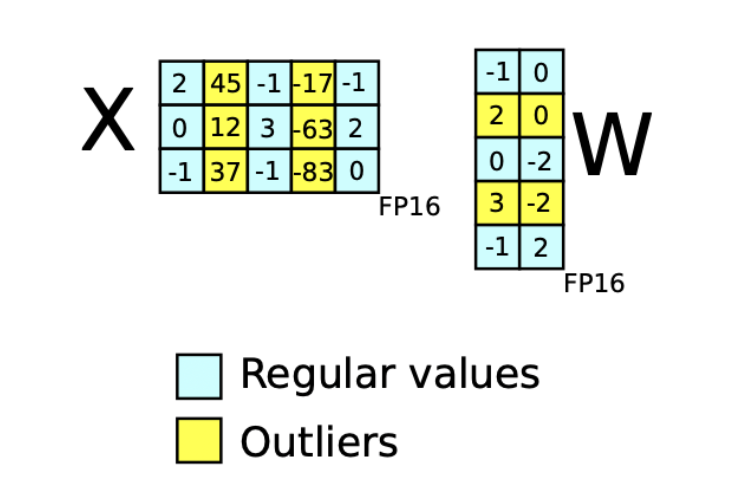
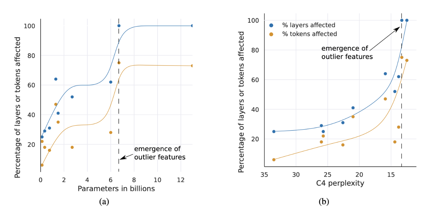
Let’s take a Transformer with \(L\) layers, whose hidden states \(X_l \in \mathbb{R}^{s \times h}\) where \(s\) is the dimension of the sequence (of tokens) and \(h\) the dimension of the features. We define a feature as a particular dimension \(h_i\) in any of the hidden states \(X_{l,i}\). Empirically, researchers track the dimensions \(h_i\) for \(i \in [[0,h]]\) that have at least one value greater than 6 (in absolute value) and collect statistics on these outliers if they appear in the same \(h_i\) dimension in at least 25% of Transformer layers and in at least 6% of all sequence dimensions \(s\) across all hidden states \(X_l\).

We then define an emergent feature as an outlier feature that appears in 100% of the layers or in at least 75% of the sequence dimensions (i.e. 75% of the number of tokens).

The result of this study is that the appearance of outlier features is systematic in large models (depending on the number of parameters, as shown in Figure 2): they appear either in most layers (i.e. they are emergent features), or in none. However, these outliers are probabilistic in smaller models: they appear from time to time in a few layers for each sequence.

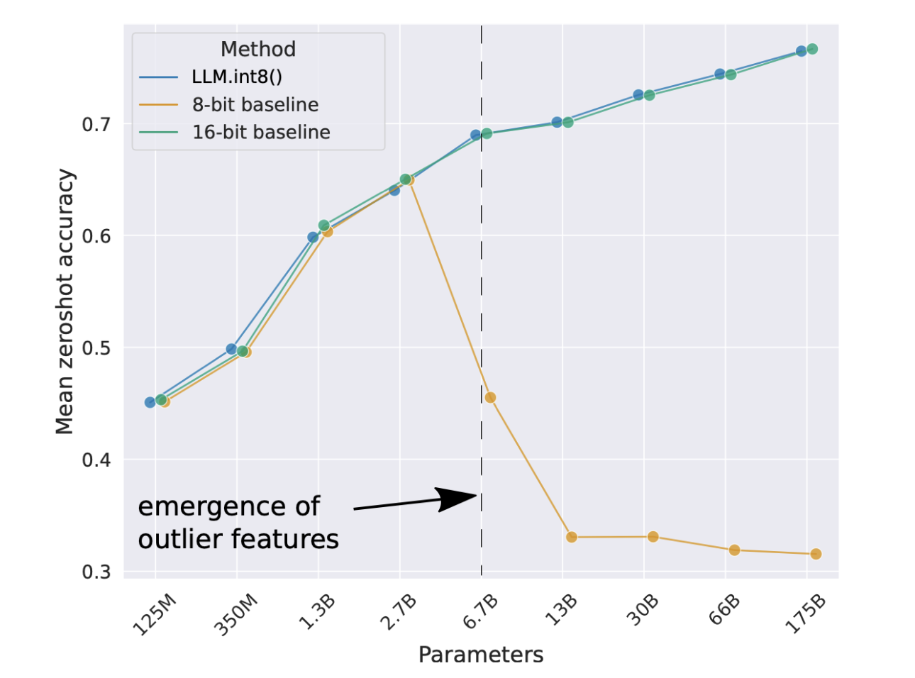
The aim of this study was to demonstrate that quantizing emergent features as if they were “regular” weights results in a very significant degradation of model capabilities. As explained above, since outlier features become emergent features around 6.7 billion parameters, it is normal to observe a degradation of models after quantization around the same number of parameters, as shown in Figure 3. The LLM.int8() publication therefore proposes quantization everywhere except on these emergent features, so as not to deteriorate model capabilities. We will follow this same logic when implementing our quantization method.

Practical application

In this section, we discuss the practical application of our project, highlighting the choice of hardware, an explanation of the quantization method chosen to adapt to its limitations, and the various resources complementing this application.

Hardware selection

To implement our Cloud Computing infrastructure, we opted for an instance hosted on Amazon Web Services (AWS) EC2 using Infrastructure as Code (detailed in appendix: \ref{anx:iac}). Given these constraints, we opted for the g4dn.2xlarge instance. This instance offers substantial computing power with 8 vCPUs and 32 GB RAM.

Quantization

As explained the previous section, LLM quantization is a complex task due to the size of the models. Indeed, it’s impossible to fully load these models to perform global post-training quantization methods, and it’s even less possible to think about re-training them, plus we have to be careful with Emergent Features so as not to increase the perplexity of the models too much. We therefore opted for a 4-bit layer-wise post-training quantization method called GPTQ, introduced in March 2023 and currently state-of-the-art in terms of LLM quantization.

Given a layer \(l\) composed of \(n\) neurons and defined by the weight matrix \(W = \begin{bmatrix} w_{1,1} & \dots & w_{1,m}\\ \vdots & \ddots & \vdots\\ w_{n,1} & \dots & w_{n,m} \end{bmatrix}\), we’ll try to convert the \(w_{i,j}\) weights into 4-bit integers, except for the emergent features.

To do this, we need to minimize the error introduced during quantization, and to know how to find the best parameters for quantization That is, to solve:

\[\begin{equation} \arg\min_{\hat{W}} ||WX - \hat{W}X||_2^{2} \label{eq:1} \end{equation}\]

where \(X_l\) represents the layer input and \(\hat{W}\) the weights after quantization.

This optimization problem is solved by following the Optimail Brain Quantization (OBQ) method \citep{Frantar2022OptimalBC} :

The first step in OBQ is to notice that this equation can be rewritten as a sum of quadratic errors on each line of \(W\), which corresponds to the MSE:

\[\begin{equation} \arg\min_{\hat{W}} \sum_{i=1}^{n}{(w_{i,:}X- \hat{w_{i,:}}X)^2} = \arg\min (\text{MSE}) \label{eq:2} \end{equation}\]

OBQ will therefore treat each line \(w_{i,:}\) independently, and quantize one weight at a time while updating the weights not yet quantized in order to compensate for the error introduced by quantizing this weight alone:

We start by fixing a line \(i\) and a random layer input \(X\), which we must solve at this stage:

\[\begin{equation} \arg \min_{\hat{w}} (wX- \hat{w}X)^2 = \arg \min_{\hat{w}} E(w) \end{equation}\]

By performing the second order Taylor expansion of this error, which we must minimize, we find:

\[\begin{equation} \label{eq:taylor} \delta E = (\frac{\partial E}{\partial w})^\top . \delta w + \frac{1}{2}\delta w^\top . H . \delta w + O(||\delta w||^3) \end{equation}\]

where \(H = \frac{\partial^2 E}{\partial w^2}\) is the Hessian matrix of the error \(E\). Noting that the neighbourhood of \(w_i\) is already a local minimum, we take the liberty of setting the first derivative to \(0\). Moreover, we neglect all orders \(\geq\) 3.

Let’s denote \(\textbf{quant}\) the function that quantizes according to the Zero-Point method. Our aim is to quantize one of the weights \(w_j\), i.e. to replace \(w_j\) by \(\text{quant}(w_j)\). This can also mean varying \(w_j\) by a quantity of \(\delta w_j = \text{quant}(w_j)-w_j\), which we can formalize as an optimization constraint:

\[\begin{equation} e_j^\top . \delta w - \text{quant}(w_j) + w_j = 0 \end{equation}\]

where \(e_j\) is the unit vector of the weight space corresponding to the scalar weight \(w_j\).

The objective is then to solve :

\[\begin{equation} \min_j \{ \min_{\delta w} (\frac{1}{2} \delta w ^\top . H . \delta w ) \space | \space e_j^\top . \delta w - \text{quant} (w_j) + w_j = 0 \} \end{equation}\]

The partial resolution of this last equation gives us the optimal update \(\delta w = \begin{pmatrix} \vdots\\ \delta w_j\\ \vdots \end{pmatrix}\) which will compensate (minimize) the introduced error \(\delta E\) during the operation \(w_j \xleftarrow{} \text{quant}(w_j)\) for any \(j\):

\[\delta w = \frac{\text{quant}(w_j) - w_j}{[H^{-1}]_{jj}} . H^{-1}.e_j\]

as well as the corresponding error:

\[\delta E = \frac{1}{2} \frac{(\text{quant}(w_j)-w_j)^2}{[H^{-1}]_{jj}}\]

I’ve left the demonstration in the appendix.

Execution acceleration

Let’s suppose that for a given line, we decide to quantize the weight \(w_q\). Let \(F\) denote the subset of weights not yet quantized. The square error has Hessian \(H_F= \frac{\partial ^2 E}{\partial w^2} = 2X_FX_F^\top\). As the Hessian depends only on X, there’s no need to recalculate it entirely. We can start from \(H\) and remove its \(q\)-th row and column (which is necessary after quantifying \(w_q\)) directly from the inverse of \(H\) by performing a Gaussian elimination:

\[\begin{equation} \label{eq:7} H^{-1}_{-q} = (H^{-1} - \frac{1}{[H^{-1}]_{qq}} . H^{-1}_{:,q} .H^{-1}_{q,:} )_{-p} \end{equation}\]

However, repeated application of this elimination accumulates numerical approximation errors, resulting in poor quantization of the layer. To address this concern, GPTQ proposes to note that the information required in \(H^{-1}_{F}\) when quantizing the \(q\) weight is contained in the elements of the \(q\)-th row, starting with the diagonal. So there’s a way of pre-calculating all these lines using a more stable method:

We note that this last step corresponds (up to a coefficient) to a Cholesky decomposition. We can therefore perform this decomposition upstream to retain all the necessary information from \(H^{-1}\). Moreover, we can speed up execution by parallelizing the quatization on a few layers at a time. In the following, we define a number \(B\) of blocks of consecutive layers on which to perform the execution.

Executing GPTQ & results

Given a matrix of weights to quantize \(W\), the Hessian matrix \(H = 2XX^\top\) and the size of a block \(B\), we quantize \(W\) following the GPTQ algorithm as follows:

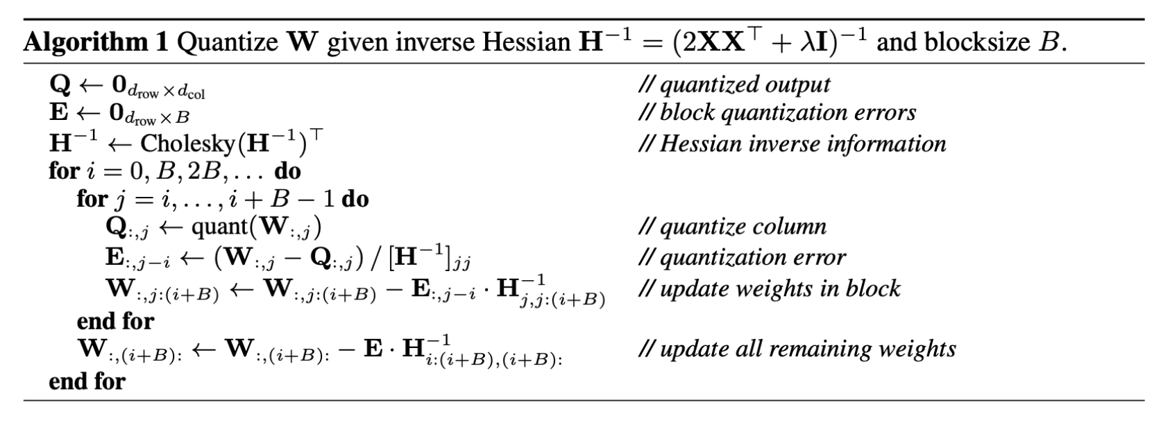
The results of this quantization are shown in Figure 4. They show a high degree of perplexity stability, even for extreme 3-bit quantizations. This stability contrasts sharply with the degradations observed with conventional methods (here the Zero-Point or Round-To-Nearest Integer method is used as a comparison, taking into account emergent features).

Pierre.

Appendix

Demonstration for the optimal update of a weight

We place ourselves at a given layer of the network, defined by the weight matrix \(W\). We fix a line \(i\) of \(W\) and look for the value \(\delta w\) corresponding to the update on the weights \(w = W_{i,:}\) which will minimize the error introduced by the quantization of \(w_j\). Starting from the Taylor expansion (4) and setting the terms of order 1 and orders greater than 3 to 0, we arrive at the following optimization problem under constraints:

\[\begin{equation} \min_{\delta w} (\frac{1}{2} \delta w^\top . H . \delta w) \quad \text{s.t.} \quad e_j^\top . \delta w - \text{quant}(w_j) + w_j = 0 \end{equation}\]

The Lagrangian of this problem is:

\[\begin{equation} \mathcal{L} = \frac{1}{2} \delta w^\top . H . \delta w + \lambda . (e_j^\top . \delta w - \text{quant}(w_j) + w_j) \end{equation}\]

The first order conditions are:

\[\begin{equation} \frac{\partial \mathcal{L}}{\partial \delta w} = H . \delta w + \lambda . e_j = 0 \end{equation}\] \[\begin{equation} \frac{\partial \mathcal{L}}{\partial \lambda} = e_j^\top . \delta w - \text{quant}(w_j) + w_j = 0 \end{equation}\]

From the first equation, we deduce:

\[\begin{equation} \delta w = -\lambda H^{-1} . e_j \end{equation}\]

By injecting this result into the second equation, we obtain:

\[\begin{equation} -\lambda e_j^\top . H^{-1} . e_j - (\text{quant}(w_j) - w_j) = 0 \end{equation}\] \[\Leftrightarrow\] \[\begin{equation} \lambda = - \frac{\text{quant}(w_j) - w_j}{e_j^\top . H^{-1} . e_j} = - \frac{\text{quant}(w_j) - w_j}{[H^{-1}]_{jj}} \end{equation}\]

Finally, we deduce the optimal update:

\[\begin{equation} \delta w = \frac{\text{quant}(w_j) - w_j}{[H^{-1}]_{jj}} . H^{-1}.e_j \end{equation}\]

References

Ganesan, K., Zhai, C., & Viegas, E. (2012). Micropinion Generation: An Unsupervised Approach to Generating Ultra-Concise Summaries of Opinions. In Proceedings of the 21st International Conference on World Wide Web (pp. 869–878). Association for Computing Machinery. https://doi.org/10.1145/2187836.2187954

Bengio, Y., Ducharme, R., Vincent, P., & Janvin, C. (2003). A Neural Probabilistic Language Model. Journal of Machine Learning Research, 3(null), 1137–1155. https://doi.org/10.5555/944919.944966

Pascanu, R., Mikolov, T., & Bengio, Y. (2012). On the difficulty of training recurrent neural networks. In International Conference on Machine Learning. https://api.semanticscholar.org/CorpusID:14650762

Hochreiter, S., & Schmidhuber, J. (1997). Long Short-Term Memory. Neural Computation, 9(8), 1735–1780. https://doi.org/10.1162/neco.1997.9.8.1735

Jozefowicz, R., Vinyals, O., Schuster, M., Shazeer, N., & Wu, Y. (2016). Exploring the limits of language modeling. arXiv preprint arXiv:1602.02410. https://api.semanticscholar.org/CorpusID:260422

Vaswani, A., Shazeer, N., Parmar, N., Uszkoreit, J., Jones, L., Gomez, A. N., Kaiser, Ł., & Polosukhin, I. (2017). Attention is All You Need. In Advances in Neural Information Processing Systems (Vol. 30). https://proceedings.neurips.cc/paper_files/paper/2017/file/3f5ee243547dee91fbd053c1c4a845aa-Paper.pdf

Devlin, J., Chang, M.-W., Lee, K., & Toutanova, K. (2019). BERT: Pre-training of Deep Bidirectional Transformers for Language Understanding. arXiv preprint arXiv:1810.04805. https://api.semanticscholar.org/CorpusID:52967399

Radford, A., & Narasimhan, K. (2018). Improving Language Understanding by Generative Pre-Training. https://api.semanticscholar.org/CorpusID:49313245

Touvron, H., Lavril, T., Izacard, G., Martinet, X., Lachaux, M.-A., Lacroix, T., Rozière, B., Goyal, N., Hambro, E., Azhar, F., Rodriguez, A., Joulin, A., Grave, E., & Lample, G. (2023). LLaMA: Open and Efficient Foundation Language Models. arXiv preprint arXiv:2302.13971. https://api.semanticscholar.org/CorpusID:257219404

Gholami, A., Kim, S., Dong, Z., Yao, Z., Mahoney, M. W., & Keutzer, K. (2021). A Survey of Quantization Methods for Efficient Neural Network Inference. arXiv preprint arXiv:2103.13630. https://api.semanticscholar.org/CorpusID:232352683

Hoefler, T., Alistarh, D., Ben-Nun, T., Dryden, N., & Peste, A. (2021). Sparsity in Deep Learning: Pruning and growth for efficient inference and training in neural networks. Journal of Machine Learning Research, 22, 241:1-241:124. https://api.semanticscholar.org/CorpusID:231740691

Nagel, M., Amjad, R. A., van Baalen, M., Louizos, C., & Blankevoort, T. (2020). Up or Down? Adaptive Rounding for Post-Training Quantization. arXiv preprint arXiv:2004.10568. https://api.semanticscholar.org/CorpusID:216056295

Yao, Z., Aminabadi, R. Y., Zhang, M., Wu, X., Li, C., & He, Y. (2022). ZeroQuant: Efficient and Affordable Post-Training Quantization for Large-Scale Transformers. arXiv preprint arXiv:2206.01861. https://api.semanticscholar.org/CorpusID:249395624

Dettmers, T., Lewis, M., Belkada, Y., & Zettlemoyer, L. (2022). LLM.int8(): 8-bit Matrix Multiplication for Transformers at Scale. arXiv preprint arXiv:2208.07339. https://api.semanticscholar.org/CorpusID:253237200

Scao, T. L., Fan, A., Akiki, C., Pavlick, E., Ilić, S., Hesslow, D., Castagné, R., Luccioni, A. S., Yvon, F., Gallé, M., & others. (2022). Bloom: A 176B-Parameter Open-Access Multilingual Language Model. arXiv preprint arXiv:2211.05100. https://api.semanticscholar.org/CorpusID:250866562

Zhang, S., Roller, S., Goyal, N., Artetxe, M., Chen, M., Chen, S., Dewan, C., Diab, M., Li, X., Lin, X. V., & others. (2022). OPT: Open Pre-trained Transformer Language Models. arXiv preprint arXiv:2205.01068. https://api.semanticscholar.org/CorpusID:248402745

Frantar, E., Ashkboos, S., Hoefler, T., & Alistarh, D. (2022). GPTQ: Accurate Post-Training Quantization for Generative Pre-trained Transformers. arXiv preprint arXiv:2210.17323. https://api.semanticscholar.org/CorpusID:253237200

Frantar, E., & Alistarh, D. (2022). Optimal Brain Compression: A Framework for Accurate Post-Training Quantization and Pruning. arXiv preprint arXiv:2208.11580. https://api.semanticscholar.org/CorpusID:251765570

Hassibi, B., Stork, D. G., & Wolff, G. J. (1993). Optimal Brain Surgeon and General Network Pruning. In IEEE International Conference on Neural Networks (Vol. 1, pp. 293-299). IEEE. https://doi.org/10.1109/ICNN.1993.298572